
Montecarlo simulation to estimate STOOIP

swimming with friends
Description
In this excercise we want to have a qualitative feel of the performance we can obtain using a Montecarlo simulation to estimate the STOOIP on a theoretical field. We will assume two extreme examples:
- Dataset 1 will have 100 samples for each parameter
- Dataset 2 will have a million samples for each parameter
In both cases we will explore the resulting distribution of Stooip and compare visually the estimation of P10, P50 and P90 running simulations that vary from 100 to a million simulations.
I will be using the followiing R packages:
STOOIP definition
The STOOIP is estimated in MM bbls with the following formula:
\[ STOOIP = Area * Thickness * Porosity * ( 1 - Sw ) / Bo * Ct \]
where:
- Area in Km2
- Thickness in meters
- Porosity in fraction
- Water Saturation in fraction
- Bo is unitless
- Ct is a constant of 6.28 to obtains mmbbls as final unit for STOOIP
Note: I have set a seed at the beginning of the code to allow for reproducibility, changing this values we can compare and realize how stable are the simulations when using different entry values.
Distributions used
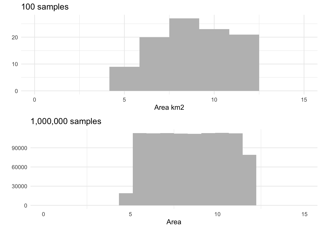
Area
The area has been set as an uniform distribution between 5 and 12 km2.
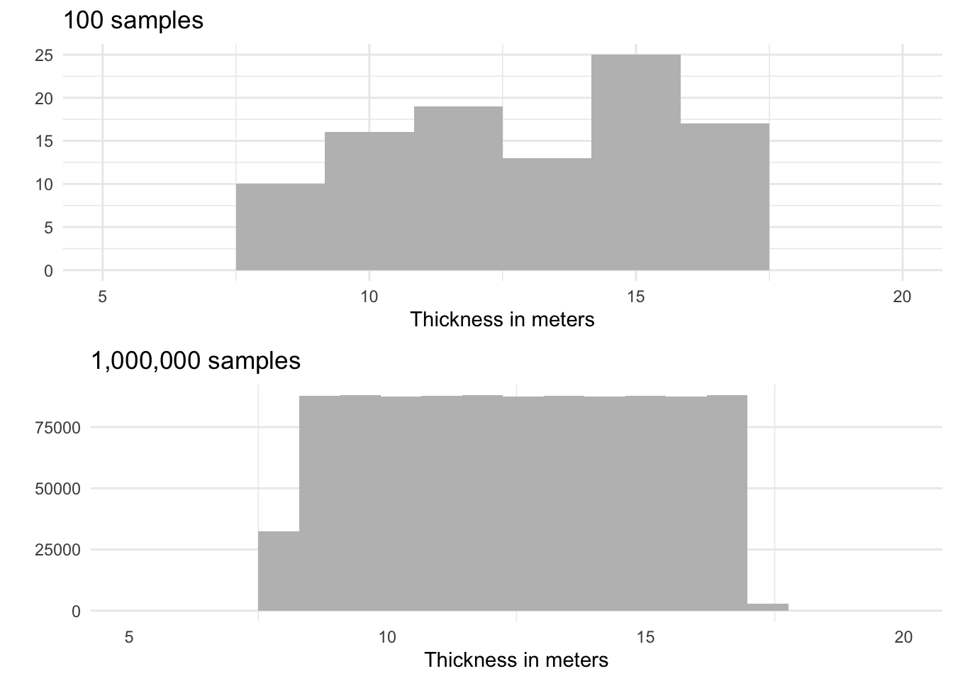
Thickness
Thickness is defined as a uniform distribution between 8 and 17 meters
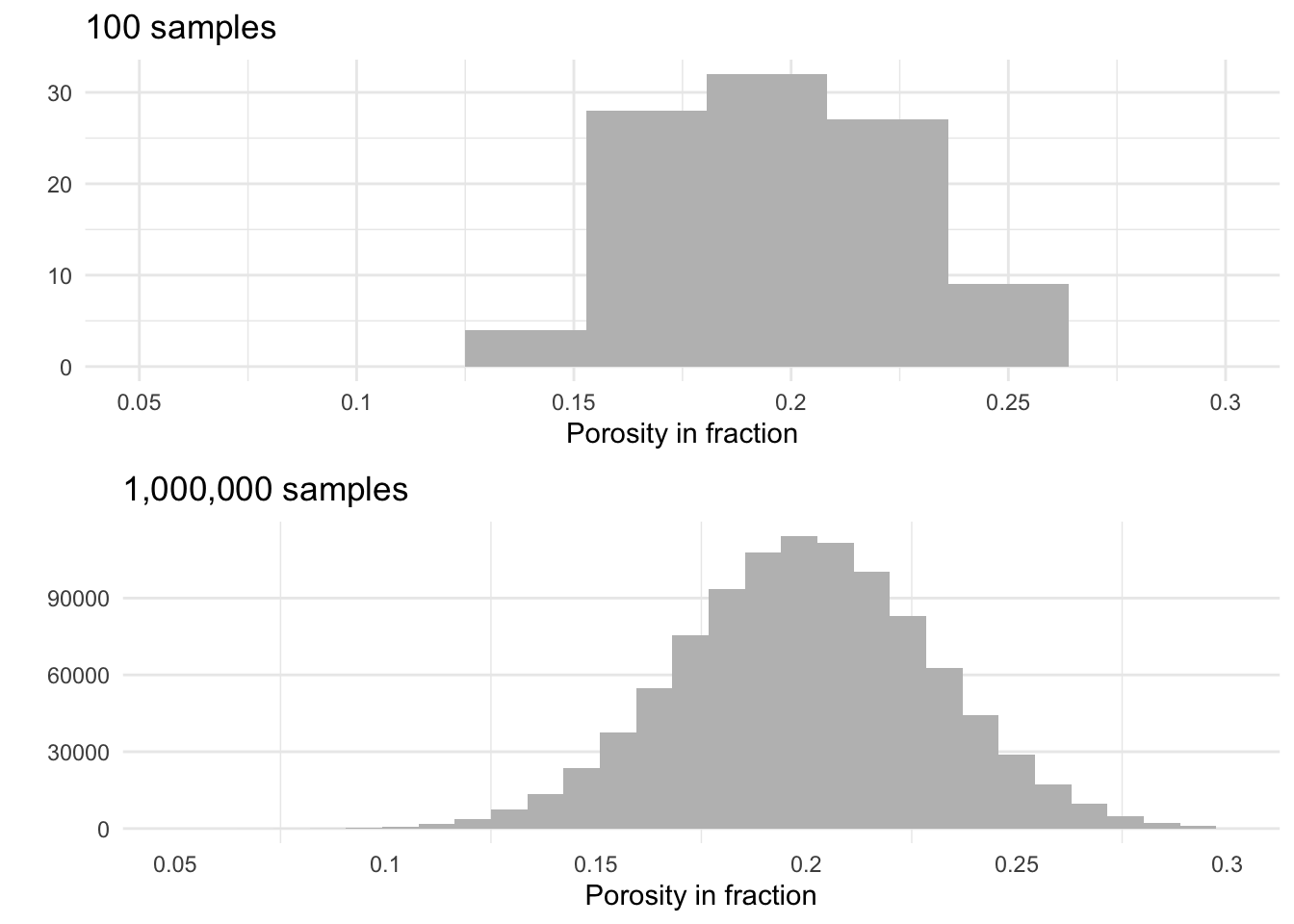
Porosity
Porosity distribution is normal with a mean of 0.2 and 0.03 standard deviation.
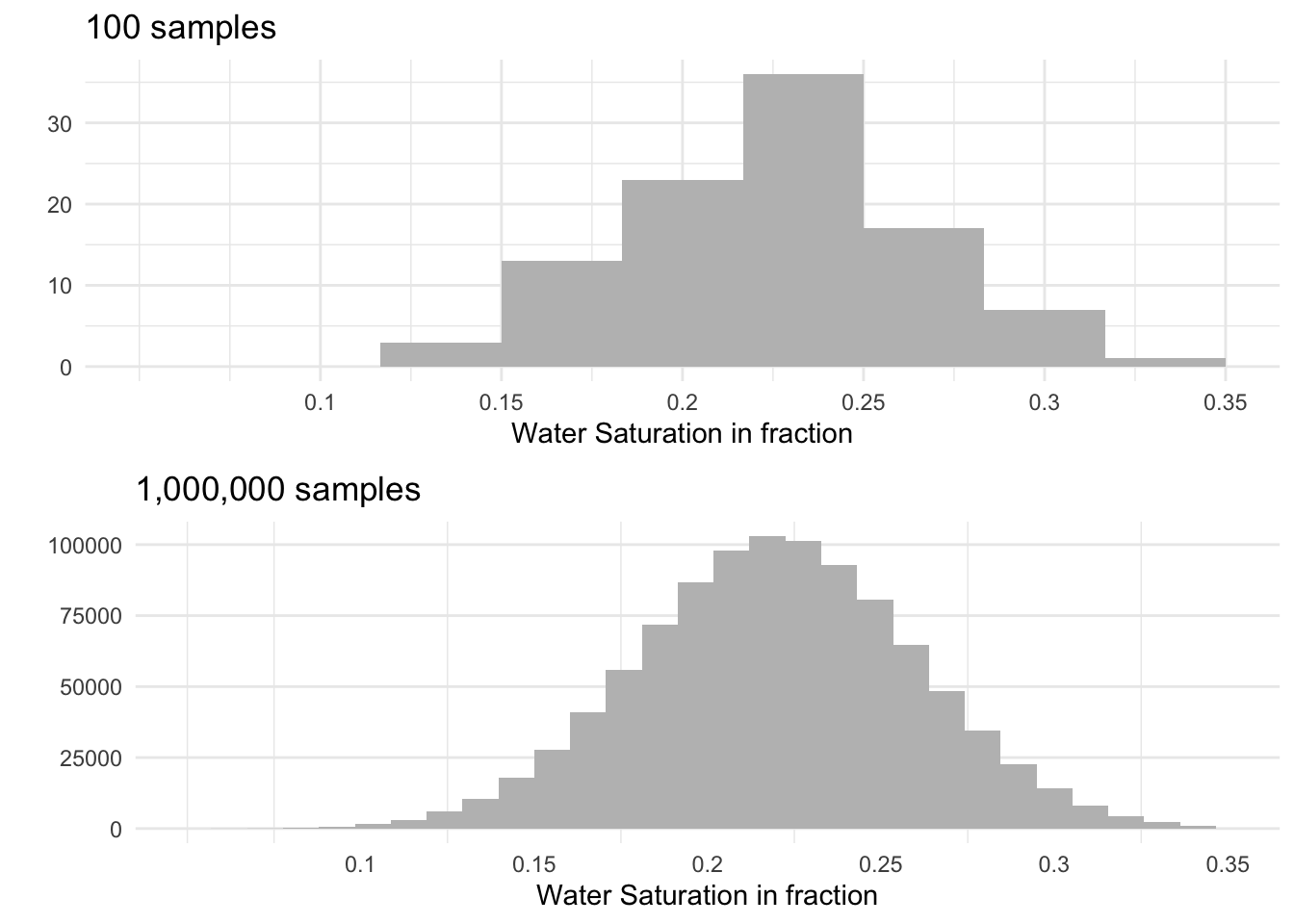
Water saturation
Water saturation distribution is normal with a mean of 0.22 and 0.04 standard deviation.
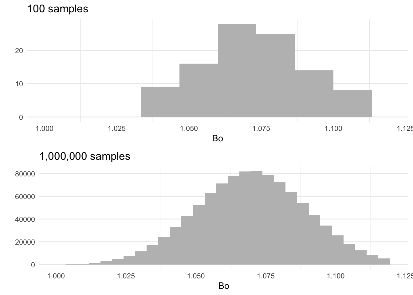
Bo
Bo distribution is normal with a mean of 1.07 and 0.02 standard deviation.
Montecarlo simulations
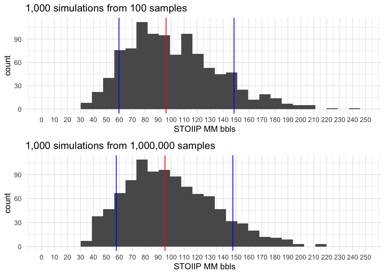
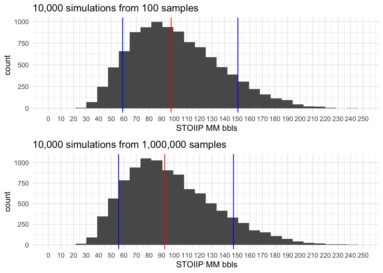
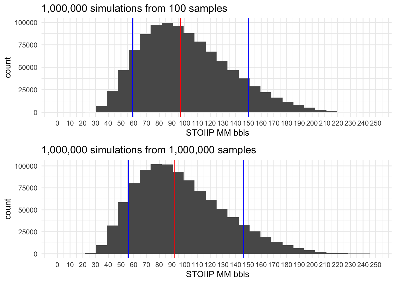
All STOOIP histograms resulting from the simulation have 3 colored lines, two Blue lines represent P10 and P90 and the Red line the P50.
100 simulations
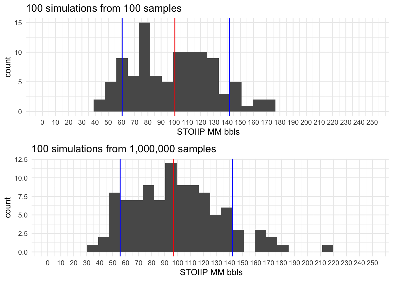
1,000 simulations
10,000 simulations
100,000 simulations
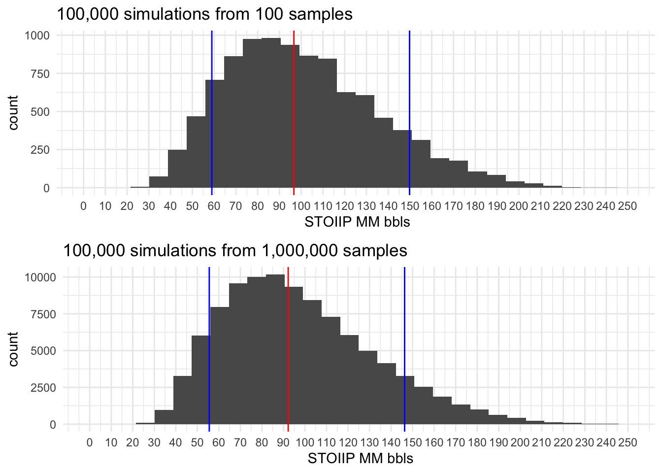
1,000,000 simulations
Conclusions
There are many conclusions to be made here, however I´will focus on the oints that normally affect my work.
- outliers or min and max values are very conditioned by the sample size, as in general in random populations we have a very small chance of capture the entire range, and this is very evident on these examples.
- the probabilities P10, P50 and P90 stabilize very early on, even with the small dataset. As usual what is good will depend on the impact this estimations will have on future decisions.